MetaTrader4
Predicting Future Prices with Neural Networks: Your Guide to BPNN
Author: gpwr
Version History:
06/26/2009 - Introduced the BPNN Predictor with Smoothing.mq4 indicator, which applies an EMA for price smoothing before making predictions.
08/20/2009 - Fixed the neuron activation function code to avoid arithmetic exceptions; updates made to BPNN.cpp and BPNN.dll.
08/21/2009 - Implemented memory clearing at the end of DLL execution; updates to BPNN.cpp and BPNN.dll.
An Overview of Neural Networks:
A neural network is a versatile model that adjusts outputs based on inputs. It consists of multiple layers:
Input Layer: Contains the initial data inputs.
Hidden Layer: Comprises processing nodes, known as neurons.
Output Layer: Consists of one or more neurons that produce the final outputs of the network.
Each node in adjacent layers is interconnected through synapses, each with a scaling coefficient called a weight (w[i][j][k]). In a Feed-Forward Neural Network (FFNN), data flows from inputs to outputs. For example, a basic FFNN might have one input layer, one output layer, and two hidden layers:
The structure of an FFNN is often expressed as: - - -...- . The example above can be referred to as a 4-3-3-1 network.
The processing by neurons occurs in two steps:
All inputs are multiplied by their respective weights and summed up.
The resulting sums are then processed through the neuron’s activation function, yielding the neuron’s output.
The activation function introduces nonlinearity into the neural network model. Without it, the network would simply be a linear autoregressive (AR) model.
The library files for NN functions allow users to select from three activation functions:
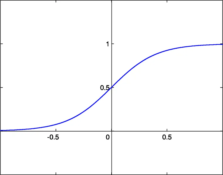
Sigmoid: sigm(x)=1/(1+exp(-x)) (#0)
Hyperbolic Tangent: tanh(x)=(1-exp(-2x))/(1+exp(-2x)) (#1)
Rational Function: x/(1+|x|) (#2)
The activation threshold for these functions is x=0. This threshold can be adjusted along the x-axis through an extra input to each neuron, known as the bias input, which also has a weight assigned.
An FFNN is fully described by the number of inputs, outputs, hidden layers, neurons in those layers, and the synapse weights. Training the network involves feeding it past input-output pairs to optimize the weights, aiming for minimal error between predicted and actual outputs. A common method for optimizing weights is back-propagation, a gradient descent technique. The provided Train() function utilizes an improved version of this method called Improved Resilient Back-Propagation Plus (iRProp+).
For more information, check out the following source: http://citeseerx.ist.psu.edu/viewdoc/summary?doi=10.1.1.17.1332
One downside of gradient-based optimization methods is that they can often get stuck in a local minimum. Given the chaotic nature of price series, the training error surface can be complex with many local minima, making a genetic algorithm a more effective training method for these scenarios.
Included Files:
BPNN.dll - Library file
BPNN.zip - Archive containing all files needed to compile BPNN.dll in C++
BPNN Predictor.mq4 - Indicator for predicting future open prices
BPNN Predictor with Smoothing.mq4 - Indicator for predicting smoothed open prices
The BPNN.cpp file contains two functions: Train() and Test(). Train() is for training the network with historical input and output values, while Test() computes outputs using the optimized weights found through training.
Here’s a brief overview of the Train() function parameters:
double inpTrain[] - Input training data (1D array carrying 2D data, oldest first)
double outTarget[] - Output target data for training (2D data as 1D array, oldest first)
double outTrain[] - Output 1D array for net outputs from training
int ntr - Number of training sets
int UEW - Use external weights for initialization (1=use extInitWt, 0=use random)
double extInitWt[] - Input array for external initial weights
double trainedWt[] - Output array for trained weights
int numLayers - Number of layers including input, hidden, and output
int lSz[] - Number of neurons in layers (lSz[0] is the number of net inputs)
int AFT - Type of neuron activation function (0:sigm, 1:tanh, 2:x/(1+x))
int OAF - 1 enables activation function for the output layer; 0 disables it
int nep - Max number of training epochs
double maxMSE - Training stops once maxMSE is reached
And here’s a brief overview of the Test() function parameters:
double inpTest[] - Input test data (2D data as a 1D array, oldest first)
double outTest[] - Output 1D array for net outputs from training
int ntt - Number of test sets
double extInitWt[] - Input array for external initial weights
int numLayers - Number of layers including input, hidden, and output
int lSz[] - Number of neurons in layers (lSz[0] is the number of net inputs)
int AFT - Type of neuron activation function (0:sigm, 1:tanh, 2:x/(1+x))
int OAF - 1 enables activation function for the output layer; 0 disables it
Whether to use the activation function in the output layer depends on the nature of the outputs. For binary outputs, typically seen in classification problems, the activation function should be used (OAF=1). However, if you’re predicting prices, you’ll want to skip the activation function in the output layer (OAF=0).
Examples of Utilizing the NN Library:
BPNN Predictor.mq4 - This script predicts future open prices based on relative price changes:
x[i]=Open[test_bar]/Open[test_bar+delay[i]]-1.0
Where delay[i] is determined through Fibonacci numbers (1,2,3,5,8,13,21..). The output of the network is the predicted relative change in the next price, with the activation function turned off in the output layer (OAF=0).
Indicator inputs include:
extern int lastBar - Last bar in the past data
extern int futBars - Number of future bars to predict
extern int numLayers - Number of layers including input, hidden & output (2..6)
extern int numInputs - Number of inputs
extern int numNeurons1 - Number of neurons in the first hidden/output layer
extern int numNeurons2 - Number of neurons in the second hidden/output layer
extern int numNeurons3 - Number of neurons in the third hidden/output layer
extern int numNeurons4 - Number of neurons in the fourth hidden/output layer
extern int numNeurons5 - Number of neurons in the fifth hidden/output layer
extern int ntr - Number of training sets
extern int nep - Maximum number of epochs
extern int maxMSEpwr - sets maxMSE=10^maxMSEpwr; training stops < maxMSE
extern int AFT - Type of activation function (0:sigm, 1:tanh, 2:x/(1+x))
The indicator displays three curves on the chart:
Red - predictions of future prices
Black - past training open prices, which served as expected outputs for the network
Blue - network outputs for training inputs
BPNN Predictor.mq4 also predicts future smoothed open prices using EMA smoothing with a defined period.
Setting it Up:
Copy the BPNN.DLL file to C:\Program Files\MetaTrader 4\experts\libraries.
In MetaTrader, navigate to Tools - Options - Expert Advisors - Allow DLL imports.
You can also compile your own DLL file using the source codes found in BPNN.zip.
Recommendations:
A network with three layers (numLayers=3: one input, one hidden, and one output layer) suffices for most scenarios. According to the Cybenko Theorem (1989), a single hidden layer can approximate any continuous multivariate function to any desired accuracy, while two hidden layers can handle discontinuous functions.
Experiment with the number of neurons in the hidden layer; common guidelines suggest using (# of inputs + # of outputs)/2 or SQRT(# of inputs * # of outputs). Keep an eye on the training error reported by the indicator in the MetaTrader experts window.
For effective generalization, the number of training sets (ntr) should be 2-5 times the total number of weights in the network. For instance, the BPNN Predictor.mq4 uses a 12-5-1 network, meaning a minimum of 142 training sets is ideal.
Ensure that input data is transformed to stationary, as forex prices are typically non-stationary. Normalizing inputs to a -1 to +1 range is also recommended.
The following graph illustrates a linear function y=b*x (x-input, y-output) with outputs affected by noise. This noise leads to a deviation in the measured outputs (black dots) from the straight line. This function can be modeled using a feed-forward neural network. However, a network with too many weights may fit the measured data perfectly, represented by the red curve, which has no relation to the original linear function y=b*x (green). This over-fitted model will result in significant errors when predicting future values due to the randomness introduced by noise.
As a token of appreciation for sharing this code, the author kindly requests that if you develop a profitable trading strategy using it, please share your insights by emailing directly at vlad1004@yahoo.com.
Good luck!
2009.06.26